Many thanks to Xavier Poncini, Paul Riechers, Fernando Rosas, and Matt Smith for useful conversations.

1. Introduction

Despite the recent successes of transformers and other sequence models, there are still many open questions about their basic principles of operation. For example, what internal representations do these models use for prediction and generation? Can we decode, interpret, and manipulate such representations? Is it even possible to consider a notion of representation without reference to an external world model?

To make progress on these questions, I propose a general way to define, decode and manipulate representations in sequence models. The approach is centered on the concept of "generalized belief states", statistics of past observations that satisfy a few criteria: (1) they are sufficient for predicting future data, (2) they can be recursively updated as new observations come in, and (3) they are low-dimensional, allowing for visualization and interpretation. I show that such generalized belief states can be mapped to the internal activations and dynamics of a sequence model, allowing for decoding and manipulation of the model's representations. I illustrate the ideas using a tractable toy model, a transformer trained on a simple HMM stochastic process, where we will see that the KV cache plays a key role.

This post is directly inspired by the 2024 paper "Transformers Represent Belief State Geometry in their Residual Stream" by Adam Shai, Paul Riechers, and collaborators. That paper introduced the idea of studying belief states in transformers, and proposed a method for doing so using tractable toy models. I recommend reading that paper if you haven't already, though it is not a prerequisite for understanding my post. Section 5 compares this approach with the one developed in that paper.

2. Belief states

We start at a general level, by considering the problem of sequence prediction. Imagine that we observe a history of previous tokens and then wish to predict the next token . We assume that sequences are drawn from a stochastic process . For now, it does not matter whether this process comes from real-world data or a generative model.

Before proceeding, we introduce a bit of notation. indicates the token alphabet, indicates the set of finite-length sequences (including the empty history ), and indicates the set of probability distributions over the alphabet . We write for the set of histories with positive probability under the stochastic process.

2.1 Hidden Markov models

To optimally predict the next token after observing history , we must compute the conditional distribution . We may now ask: what information should we track in order to compute this distribution? How should this information be updated as new tokens arrive? Does this information represent some unobserved latent aspect of the stochastic process?

These questions have a straightforward answer when the stochastic process is described as the output of a hidden Markov model (HMM). Given an HMM description, we can write the probability of any history as ^[1] where is the hidden state of the HMM at step , is the probability of emitting token and transitioning to hidden state from hidden state , and is the initial distribution over hidden states. Using this expression and Bayes' rule, the next-token distribution can be written in a factorized form as Here, is the Bayesian posterior distribution over the hidden state, conditioned on the observed history . This posterior distribution corresponds to the beliefs of a Bayesian observer about the underlying states of the generating process, and in the literature, it is called a belief state. ^[2]

Belief states satisfy two important properties: sufficiency and recurrence. Sufficiency means that the belief state allows us to predict the next token just as well as if we knew the whole history , as seen from the prediction map in Eq. (1a). Recurrence means that, after observing a new token , the updated belief state can be computed from and alone. In particular, using Bayes' rule, we can write the update map as

In addition to sufficiency and recurrence, belief states have several other attractive properties. For instance, the prediction map (1a) is time-independent and linear in . Time-independence lets us interpret belief states at different steps in the same way; linearity lets us interpret predictions as convex mixtures of those made by individual hidden states. The update map (1b) is also time-independent and "nearly" linear, being a ratio of two linear functions of the belief state. (In fact, without loss of generality, we may instead consider "unnormalized" belief states , which update in a purely linear way . ^[3] )

In practice, belief states are often encoded as nonnegative vectors: where is the number of hidden states of the HMM. In this way, each belief state is a nonnegative -dimensional vector that sums to 1, so it belongs to a -dimensional affine subspace of . For HMMs with few hidden states, belief states belong to a low-dimensional space, allowing for easy visualization and interpretation. Also, in this space, belief states often exhibit a remarkable fractal structure, which arises from the recursive nature of the update map. ^[4]

2.2 Example

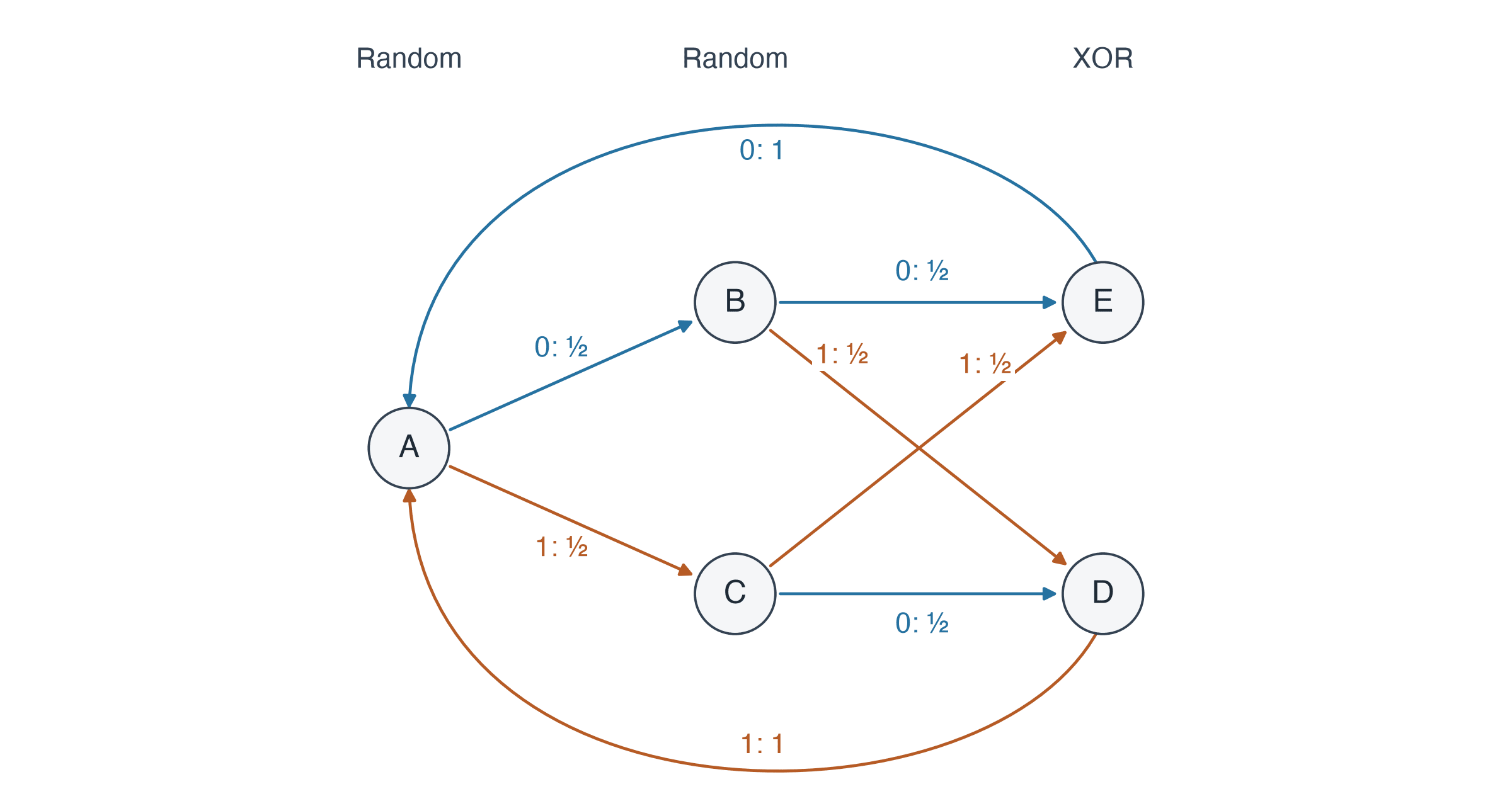
To make things concrete, we now introduce a running example: a stochastic process called MRRXOR that is generated by an HMM with five hidden states. ^[5] The HMM emits two independent random bits, then their XOR, and then resets. In addition, at each time point, the hidden state can jump to another random hidden state with probability ; if this random jump occurs, it does not emit a token and is immediately followed by an ordinary transition. The HMM is shown in the following figure, with each transition labeled by its emitted bit and probability. (For visual clarity, the random jumps between hidden states are not shown.)

Next, we illustrate the geometry of belief states for this HMM. We compute the belief states after each of the possible histories of length . Each belief state is a normalized nonnegative vector that belongs to a four-dimensional affine hyperplane of .

We visualize these vectors using principal component analysis (PCA), showing all six pairs of the four non-trivial principal components. Each belief state is colored by the last two tokens of the history, with its point area proportional to the history probability. Black dots correspond to each of the five hidden states A–E.

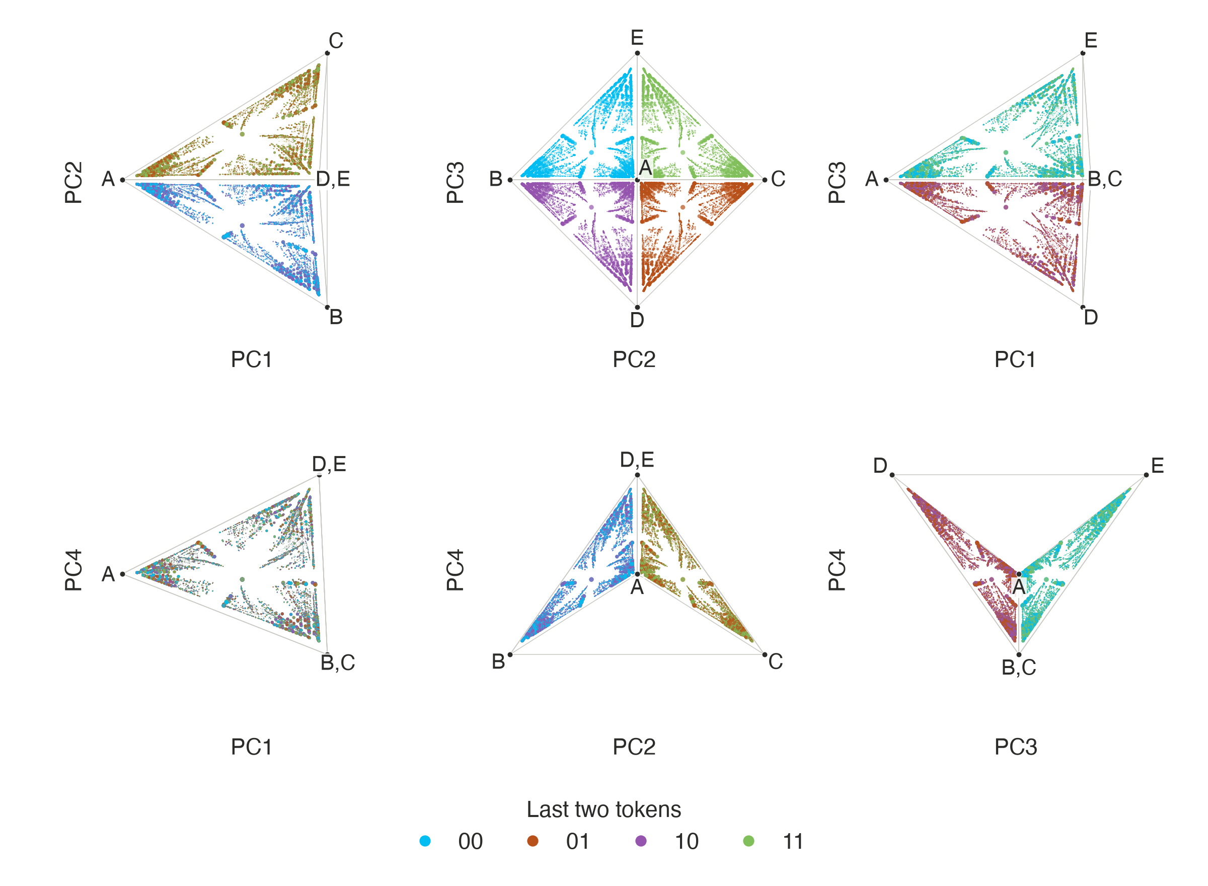
PC1 largely tracks the probability of the "reset" state A, i.e., the belief that an XOR triple has just been completed. PC2 separates histories by their last token. PC3 s